Unsupervised Learning – K-means Clustering

Clustering is a kind of unsupervised learning where we try to identify similarities and patterns from unlabeled data. Data points which exhibit similarities are grouped together into a cluster, and there is no fixed way these data points can be separated — clustering is subjective. Ideally, good clusters will exhibit high intra-class similarity and low inter-class similarity. This would mean that the maximum distance between points within a cluster will be small, but the distance between clusters is large. There are several ways to determine similarity, which shall be covered in a separate blog post.

What is K-means Clustering?

• It uses a Partitional Clustering approach, as opposed to hierarchical clustering. This means that the data is divided into various partitions according to some criterion
• Each cluster is associated with usually a randomly chosen centroid, which is the average of all the data points in that cluster, and does not have to be an actual data point. Compare this to medoids, which is the most representative data point in the centre of the cluster. There is another algorithm that bases each cluster around a medoid, called the k-medoids clustering
• Each point is assigned to a cluster according to how close it is to the centroids, where closeness can be measured by Euclidean distance, cosine similarity, correlation, etc
• Number of clusters must be specified. This is where it becomes tricky because you wouldn’t be so sure how many clusters there should be, given that it’s unlabeled data. One way to decide the number of clusters would be to start with a large number, and then select the centroids that are furthest from each other. Another way would be to use the bisecting K-means algorithm

Limitations of K-means Clustering

• Clusters are not globular, or are not of similar size/density
• Data contains outliers

I’m going to try K-means clustering on the glass dataset available here in R.
Here’s a description of the attributes in the dataset taken from the UC Irvine site:

Attribute Information:
1. Id number: 1 to 214
2. RI: refractive index
3. Na: Sodium (unit measurement: weight percent in corresponding oxide, as are attributes 4-10)
4. Mg: Magnesium
5. Al: Aluminum
6. Si: Silicon
7. K: Potassium
8. Ca: Calcium
9. Ba: Barium
10. Fe: Iron
11. Type of glass: (class attribute)
— 1 building_windows_float_processed
— 2 building_windows_non_float_processed
— 3 vehicle_windows_float_processed
— 4 vehicle_windows_non_float_processed (none in this database)
— 5 containers
— 6 tableware
— 7 headlamps

glass <- read.csv("glass.data", header=FALSE) #6 classes

#Remove label
x <- glass[-c(1,11)]

#Cluster unlabeled data
cl<- kmeans(x,6)

#print out the results
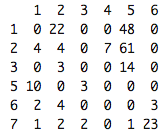
table(glass[,11],cl$cluster)

The row names represent the classes in the dataset, and the column names represent the clusters.
As can be seen from the table, the clusters aren’t capturing each class well (for eg class 1 is split between cluster 2 and 5 and lots of data points are falling in cluster 5). The accuracy rate is 0.7477.

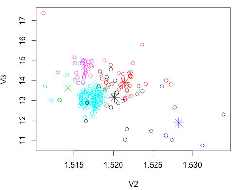
Below is a plot of the 6 clusters and their centroids with the first 2 attributes.

plot(x[c("V2", "V3")], col=cl$cluster)
points(cl$centers[,c("V2", "V3")], col=1:6, pch=8, cex=2)

The centroids are marked with an asterisk, and the data points are colored by clusters.

Out of curiosity, let’s try normalizing the data to see if it improves the accuracy rate of the clustering. Normalizing the data will transform the data such that mean = 0 and standard deviation = 1.

#re-run k-means with scaled data
xscaled <- scale(x)
cl2 <- kmeans(xscaled,6)

Interestingly, the accuracy rate for the scaled dataset dropped to 0.5561.

Now let’s try the Bisecting K-means algorithm on the unscaled glass data.

What is the Bisecting K-means Algorithm?

• Select a cluster to split
• Use the basic k-means algorithm to split the cluster into 2 sub-clusters. Do this for the number of iterations chosen
• Add the two sub-clusters with the lowest SSE to the list of clusters
• Continue until you obtain your desired number of clusters

Below is my attempt to write a wrapper for the inbuilt kmeans() function in R such that it will implement the Bisecting K-means algorithm. Although it is known that there are 6 classes in this dataset, I am going to proceed by assuming that the number of classes is unknown so that I have to determine the number of clusters necessary.

#Find the desired number of clusters
nclust <- function(x, maxclust=15) {
  wss <- (nrow(x)-1)*sum(apply(x,2,var))
  for (i in 2:maxclust) wss[i] <- sum(kmeans(x, centers=i)$withinss) 
  plot(1:15, wss, type="b", 
       xlab="Number of Clusters", 
       ylab="Within groups sum of squares")
}

nclust(x)

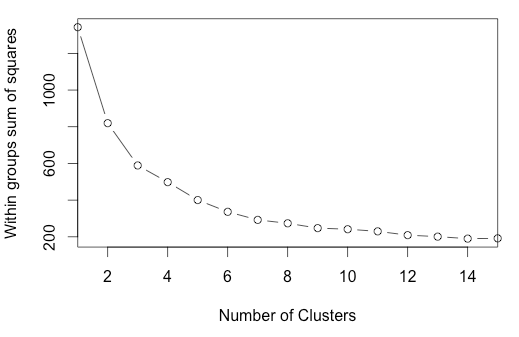
The above plots the Sum of Squared Errors (SSE) for increasing number of clusters. There seems to be a slight elbow at numClusters = 3, but it is not very clear.

library(fpc)
pamk.best <- pamk(mydata) #suggests 3 again
pamk.best$nc

pamk.best$nc
[1] 3

Again, even with the fpc package, it suggests that the optimal number of clusters should be 3 and so I will go ahead with numClusters = 3.

ss <- 1000000
cl <- kmeans(x,2) #initial kmeans splits data into 2 clusters
tosplit <- which(cl$withinss == max(cl$withinss)) #further split the cluster that has higher within cluster sum of squares into 2 sub-clusters
rows <- which(cl$cluster == tosplit)
splitClust <- x[rows,]
index1 <- which(cl$cluster != tosplit)
answers <- glass
answers[index1,12] <- 3

bestClust = function (myData, numClusters = 2) {
  for(i in 1:100) { #100 iterations
    cl2 <- kmeans(myData,2)
    if(mean(cl2$withinss)<=ss){ 
      ss<- mean(cl2$withinss) #set ss to the lower avg
      cl2.best<-cl2 #set model with lower ss as best model
    }
  }
  return(cl2.best)
}
cl3 <- bestClust(splitClust,2)
answers[-index1,12] <- cl3$cluster
table(answers[,11],answers[,12])

Looking at the results of this table, we see that both class 1 and class 3 were perfectly assigned to cluster 3. This might be due to how class 1 and class 3 were both “float-processed” glass.
Class 5 (containers) and Class 6 (tableware) were not clustered well. Majority of Class 7 (headlamps) was captured in Cluster 2.

Since the glass dataset was originally used to determine if a glass type was of “float” glass or not, we will consider Class 1 and Class 3 as correctly assigned into a cluster as they are both of “float” type.
The accuracy rate of this would be then 0.5654

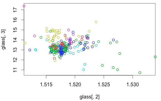
#visualize test of first 2 attributes
plot(glass[,2], glass[,3])
points(glass[which(glass[,11] == 1),2:3],col = 4) #blue
points(glass[which(glass[,11] == 2),2:3],col = 3) #green
points(glass[which(glass[,11] == 3),2:3],col = 2) #red
points(glass[which(glass[,11] == 5),2:3],col = 5) #turquoise
points(glass[which(glass[,11] == 6),2:3], col = 6) #fuchsia
points(glass[which(glass[,11] == 7), 2:3], col = 7) #yellow

Referring to the graph, we can see that Class 1 (blue), Class 2 (green) and Class 3 (red) are highly overlapping. Class 5 (turquoise) and Class 6 (fuchsia) had few data points but covered a wide range, which was probably why there was high error rates for these 2 classes.